

Background
Resource Optimized Placement (ROP)
A while back, I've published an article for Resource-based placement with cooperative dual-mode Kalman filtering. This made it into Orleans under a slighlty different name: Resource Optimized Placement.
It essentially is a placement strategy which attempts to optimize resource utilization across the cluster by means of placing new grain activations as they come in.
You can read more about ROP here.
Locality-aware Activation Repartitioning (LAR)
A few of the community members reported that ROP resulted in an improved utilization of resources in a cluster. This was a great win, but achiving optimal resource utilization is a very hard problem, due to so many factors at play.
Surely ROP did its part, but memory & CPU usage are not the only variables that lurke around! A major factor is latency that arises from network jumps when any two activations talk to each other.
While ROP did some work around favoring (at a certain degree) local placements, it just could not (and was never meant to) cope with the highly-dynamic nature of grain deactivation and reactivation. I like to draw parallels between distributed systems and chaotic systems.
With time, any non-trivial distributed system, will go off the rails, and continuous readjustments are neccessary! The burden put on any distributed system, especially an actor-based one, is very apparent.
There was a need to co-locate highly-interconnected (chatty) activations, and LAR was born out of that need. LAR was inspired heavily from Optimizing Distributed Actor Systems for Dynamic Interactive Services, and while it did adhere to it for most of the part, at the end, way more strategies and algorithms were introduced in order for the solution to not crumbled upon itself during high load.
In a nutshell, LAR collocates activations based on observed communication patterns to improve performance, while keeping the cluster balanced. The initial benchmarks, showed throughput improvements in the range of 30% to 110%. This is being conservative as it performs better (relative to it being off) the more chaotic and randomly distributed the system is.
You can read more about LAR here.
Memory-aware Activation Rebalancing (MAR)
ROP is focused on placing new activations in a way that tries to achive maximal balance in terms of resource utilization.
LAR is focused on co-locating chatty activations, and essentially break remote connections and transform them into local once, all this while respecting a tolerance level for imbalance (which is configurable).
I have seen some (rightfully so) confusion towards LAR, and parts of it (I think) may arise from my initial naming of it as "Active Rebalancing". I want to clear that out now that LAR does NOT rebalance! That is not its focus, and it can NOT do that.
The best it can do on that front, is to try to keep whatever imbalance there is, under the threshold limit mentioned above. That imbalance is based on activations between any two exchanging silos, and while an "activation" is a good proxy for resource utilization, nevertheless its not perfect.
There is a need for a another functionality, one that is concerned specifically with rebalancing of activations. A functionality that is adaptive, can run automatically but also desirably on-demand.
In a wide spectrum, once a system is balanced, and the dynamics of the system is fairly stable, the system will remain balanced (given some error margin).
A cluster of silos, is mostly imbalanced during deployments, specifically a rolling-upgrade style of deployment. But as mentioned with the parallels drawn to a chaotic system, it is unpredictable how a system evolves, as it depends on so many factors (business logic, and peak-hours being large contributors).
In the rest of this article, we will explore a novel approach to achiving Adaptive Rebalancing. We will approach this by:
- Starting with first principles.
- Build upon those and try to rigorously derive optimality conditions.
- Put those into test via simulations.
- Look back and refine.
Introduction
We are given a cluster of S silos, and that number is likely variable with time. We know the total number of activations which we try to distribute in some way that is deemed "optimal".
- How do we know the system is balanced / imbalanced?
- How do we decide which activations to move, and where?
- How do we decide how long the process of rebalancing lasts?
- What is even considered "optimal"?
Equilibrium and Entropy
When you have a problem that is considered "hard", one should look at nature and ask himself
How does nature deal with this?
A thermodynamic equilibrium is a state where a system's macroscopic properties remain constant over time, this is characterized by the principle of maximum entropy.
Entropy, a measure of disorder or randomness, naturally increases as a system evolves towards equilibrium. This principle is governed by the second law of thermodynamics, which states that the total entropy of an isolated system can never decrease.
In practical terms, this means that energy and particles within a system (typically an isolated gas container) will distribute themselves in a manner that maximizes entropy, resulting in a stable and balanced state.
Similarly, in a distributed actor system like Orleans, achieving equilibrium involves finding the optimal distribution of activations (think of them as gas particles) across various nodes or silos.
Just as particles in a gas container move towards a state of maximum entropy, activations within a cluster can be redistributed to maximize the overall cluster's entropy. By treating the cluster as a unified entity, we can apply the principle of maximum entropy to ensure a balanced load distribution, thereby enhancing system efficiency and performance.
Look at the picture below, we can see a big container which is separated by faint lines representing silo boundaries. Each of the silos host a different number of activations. The boundaries are sepparated intentionally with faint color to showcase that for equilibrium analysis, the boundaries do not matter.
The cluster is composed out of 5 silos, having: 10, 30, 120, 290, and 50 activations, respectively. We can visually observe that the distribution of activations is non-uniform.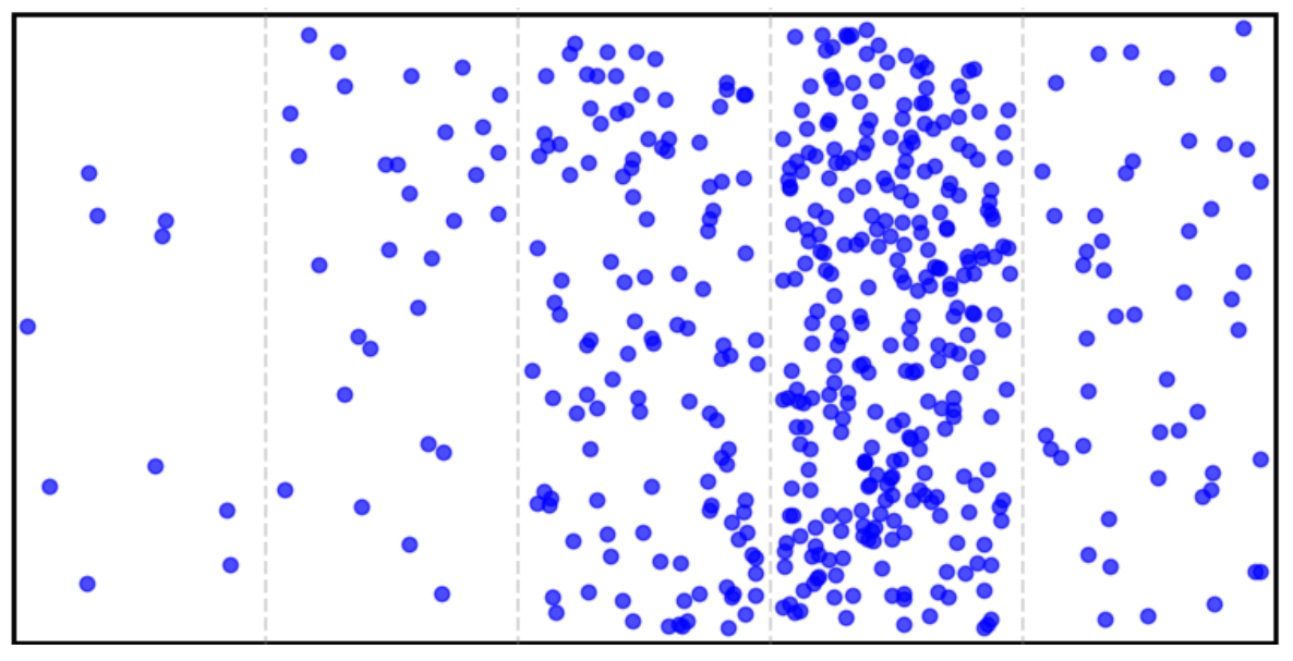
Below we see the same cluster of 5 silos, this time each of them having 100 activations. We can visually observe that the distribution of activations is uniform.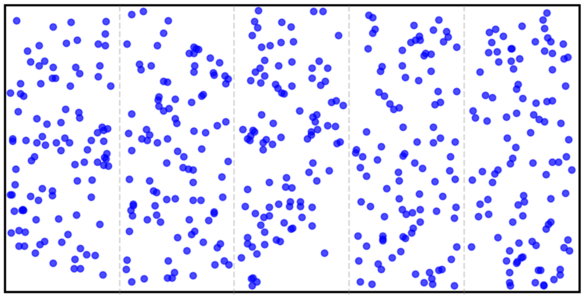
Information Entropy
The principle of maximum entropy (thermodynamic equilibrium) while it sheds a great deal of light into approaching our problem, the actual formula for entropy in the theory of statistical mechanics:
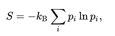
is not quite suited, as we are not dealing with gas particles, but with logical entities of information i.e. grains. Interestingly the Gibbs formula for entropy in statistical mechanics is a special case of the deeper and more fundamental information entropy, also known as Shannon Entropy, given by: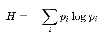
Where pi is the probability distribution, or given our discrete nature of the problem, more precisely the mass density function.
Entropy H in this context can be defined as a measure of the distribution of activations across silos. The entropy of the cluster at any given point in time can be defined as:
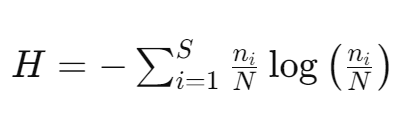
pi = ni / N being the probability of an activation being in silo i. This can be interpreted as:
The higher the number of activations is at silo i, the higher the chance of finding an activation there.
Information equilibrium in this context means that the cluster's state (distribution of activations) must change in such a way to maximize entropy until it reaches a certain distribution.
Activation Constraint
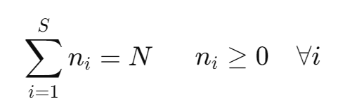
When searching for the distribution function that maximizes entropy, we need to put the system under one or more constraints. The most sensible constraint in the context of activation balancing is:
The sum of activations in all silos must equal the total number of activations in the cluster. The number of activations in any silo cannot be negative.
Proof
Given that pi = ni / N is the probability of an activation being in silo i. The sum of all probabilities must equal to 1:
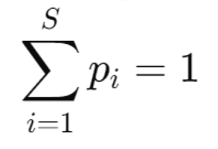
Substituting ni / N for pi, and since N is independent of the sum index, we end up with:
Lagrange Multipliers
Since we want to find the distribution function that maximizes entropy, this immediately tells us that we are dealing with an optimization problem.
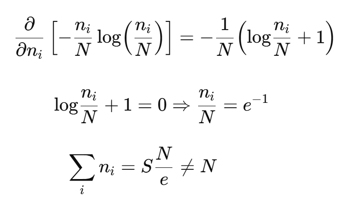
In calculus, in order to find the maximum (or minimum) of a function, we take the derivative of it and equate it to zero. Technically this gives us the optimum of the function but ignores any given constraints, leading to an incorrect answer!
In order to account for the constraints, we use the method of Lagrange multipliers, given by the general form:
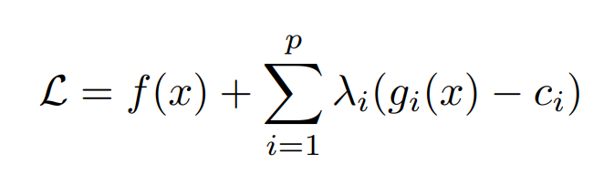
Where λ1 , .. , λp are new variables that we introduce into the system, and gi(x) are our constraining functions, and ci are all the right-hand sides of the constraining functions gi(x).
In order to find the optimal, or rather the stationary point(s), we take the partial derivatives with respect to: x, λ1 , .. , λp and equate them to zero.
From there on, we have a system of equations which (if lucky) are a set of linear equations, and we can find a closed-form solution (after which we are after).
Cluster Entropy Maximization
Given the equation for information entropy and our constraint on the cluster, we can write down the Lagrangian for our system:
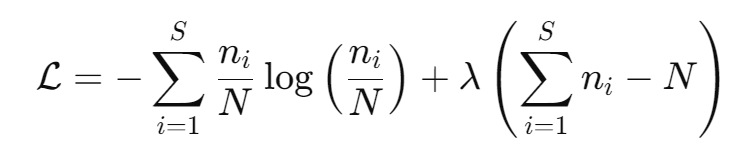
Note that taking the partial derivatives and equating to zero, results in stationary point(s) in such a way that the maximum does not mean a "true" maximum, but a point that is considered a "maximum" given the constraint.
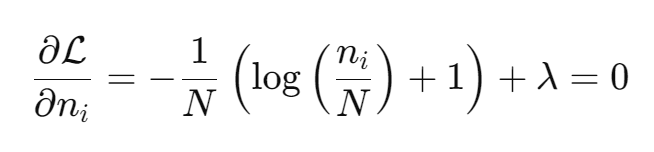
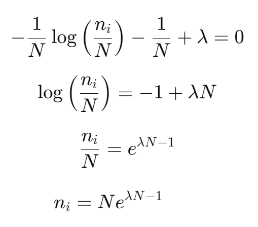
When taking the partial derivative of ℒ with respect to ni, the expression under the derivative is a sum from i = 1, ... S, but we are taking the derivative with respect to the ith n, therefor all other terms nj (for j != i) are constant and their derivative are zero. The same applies for the second term, and the derivative with respect to the ith n is simply the langrage multipler λ itself.
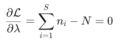
When taking the partial derivative of ℒ with respect to λ, the first term becomes zero as it is not depended on λ. This time the sum stays as the derivative does not operate on any ni.
From the first equation we solve for ni:
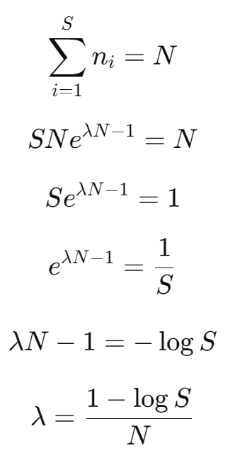
We substitute the above result for ni into our constraint, and solve for λ:
Substituting λ back into the equation for ni we get:
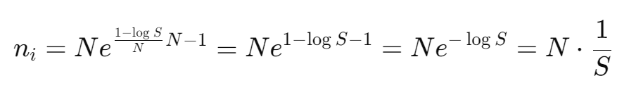
Which indeed is our activation distribution function, that results in maximum entroy. And it should be apparent that this distribution function is the uniform distribution.
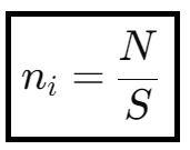
We arrived at a closed-form solution for ni, which is a uniform distribution, which means that balance is achived when every silo has N / S activations. The maximum entropy for a perfectly balanced system (where ni = N / S, for all i) thus can be calculated as:
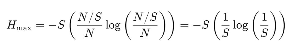
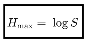
This provides us with a metric or rather a reference point in order to find out how much balanced / imbalanced the cluster is at any given time. Because we can compare the current entropy with the maximum entropy.
At any given balancing cycle, some component (the most logical is a silo) takes the responsibility of determining the current and maximum entropy of the cluster. This responsibility can freely be transferred to any other silo (or something else).
Technically the maximum entropy does not change if the number of silos says the same, but the algorithm inherently supports a dynamic cluster (which is important during rolling upgrades).
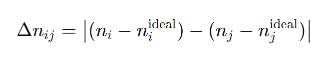
Silos form pairs in such a way that each pair, has a number of activations that are maximally apart from each other. For each such pair, we compute the absolute value of the difference of the deviations from the ideal activation count (determined by our distribution function):
Let α be the ratio between the current entropy and the maximum entropy:
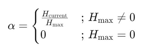
α can act as a progress indicator, but more importantly it represents the aggressiveness towards the number of migrations to determine. Given an initial low-entropy cluster, α is relatively low to being with, as the current entropy is much lower than the maximum, but with every cycle the cluster converges towards equilibrium, at which point α = 1.
This tells us that the balancing starts off conservatively (due to higher risk of cluster disruptions), but as the cluster converges to the balance, every migration batch has lower chances of disruptions, as naturally the batches becomes smaller, therefor any deviation difference is scaled less than the previous one. This is true with higher number of silos, but as we shall see, more work needs to be done to support clusters with a relatively low number of silos.
Note that α can vary as the number of silos changes while AR is at play. Nevertheless, the system reacts accordingly at any point. Therefor the adjustment delta 𝝳n is given by:
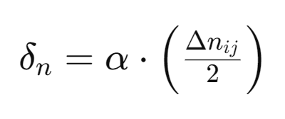
We average the deviation difference to ensures that no silo makes a disproportionately large adjustment in one cycle. By averaging we minimize the variance i.e. how spread-out from equilibrium the activations are. We divide by 2 because it is two silos being compared.
Simulations
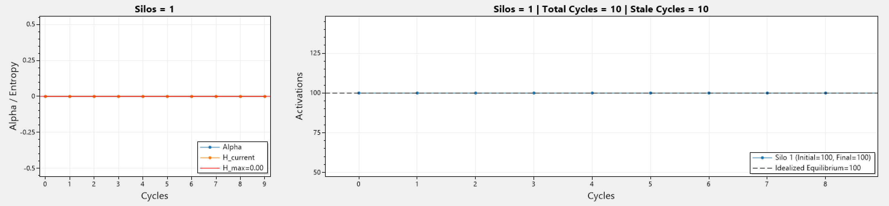
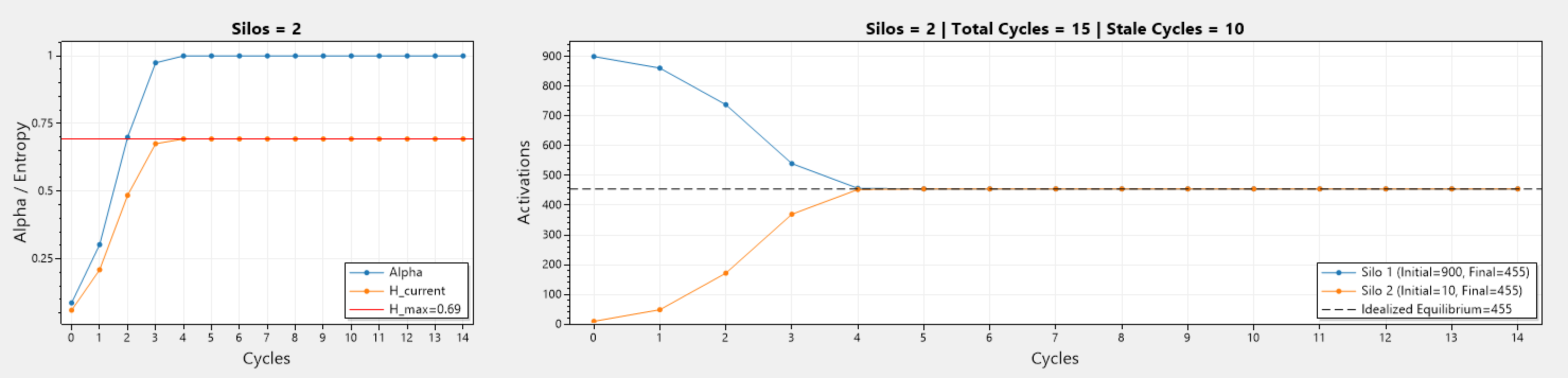
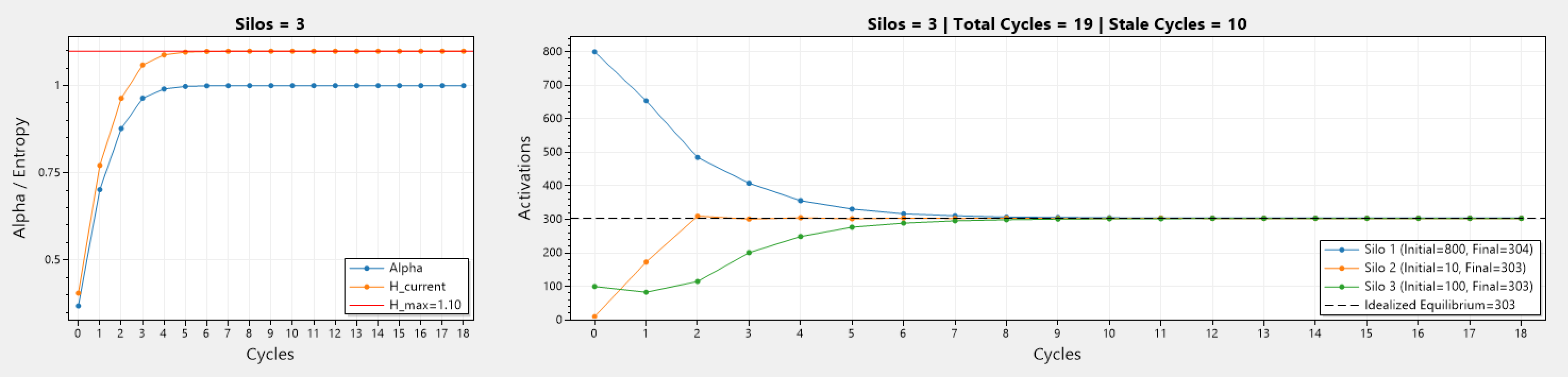
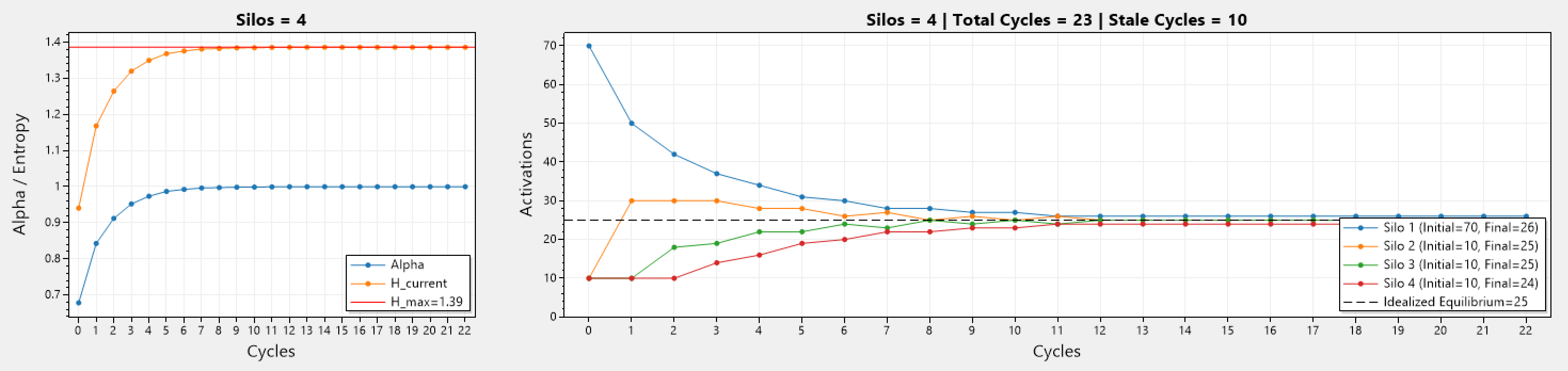
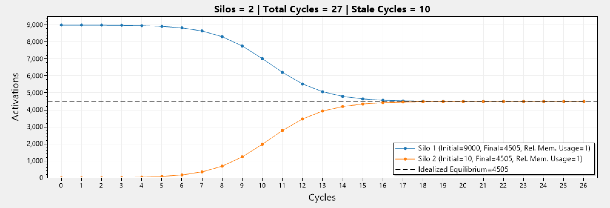
Above we can see a series of simulations involving different number of silos, and different initial number of activations.
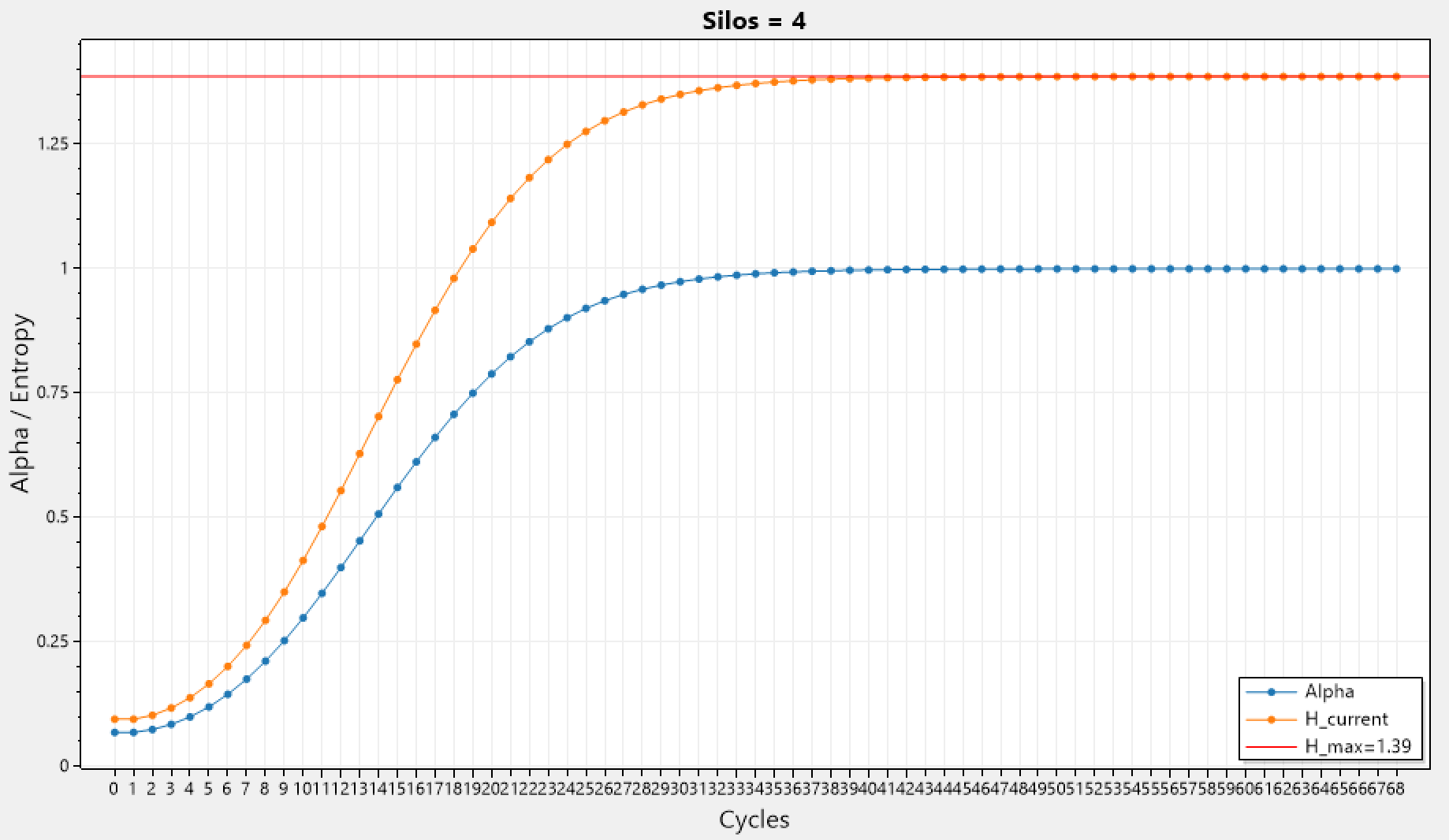
The left graph depicts how the current entropy H_current changes during each cycle, while the maximum entropy H_max stays consistent as these simulation represent a static cluster (mainly because the simulation code was getting quite complex). In addition, α which is the ratio between H_Current / H_Max, also changes and trends towards 1, and becomes 1 when H_current = H_max.
The right graph depicts how the number of activations changes over the cycles. Silos start with different activations, and as cycles go past, the activation count in all silos trend towards the idealized equilibrium (denoted by ---). Simulations run until equilibrium is reached, or if x consecutive cycles yield no improvement to the current entropy.
On the first graph, there is only a single silo, therefor all: α, H_current, and H_max, are equal to 0. While the right graph shows no changes to the number of activations in the silo (they can not go anywhere else). Note that this is actually the algorithm running, and not hard-coded values!
The other graphs involve 2 or more silos, therefor AR can operate. The important thing to note is that with more silos, the number of cycles until equilibrium is reached grows, which is to be expected.
Memory Constraint
The above equations (therefor also the simulations), do not take into account memory usage of the involved silos, which is not ideal in the real world, so the question is:
How do we incorporate memory usage into the distribution and maximum entropy equations?
One would assume a linear relationship between the number of activations and the memory usage, which would yield to simply adding an additional constraint on the Lagrangian, but that would be incorrect. While true that there is a proportional relationship between the two, it is not linear, because that would imply that any change in the number of activations would yield to a linear change in memory usage, which is not true.
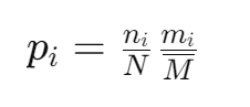
Let pi be the new probability distribution. This time the probabilty that we can find an activation on silo i is proportional to the number of activations at silo i, but also proportional to the memory usage at that silo. This can be interpreted as:
The higher the number of activations, and the memory usage at silo i, the higher the chance of finding an activation there.
The probability of finding an activation in silo i this time is higher than on the activation-only constraint, and it makes sense, as a silo with higher number of activations and higher memory usage, has a higher chance of hosting an activation, as opposed to one with less of those quantities.
But the probability function must always be dimensionless, and mi has units of bytes (in practice that would be multiples of it), therefor we need to normalize it by dividing by the average memory usage Mm.
In order to accomodate for possibly very different memory usage patterns across the cluster, we will use the harmonic mean as our memory mean.
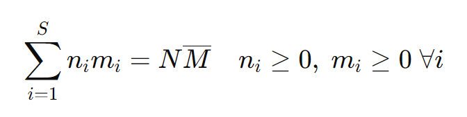
We shall establish the new constraint as:
The sum, of the products between activations and memory usage in all silos, must equal the product of the total number of activations and the mean memory usage in the cluster. The number of activations and memory usage in any silo cannot be negative.
Proof
Given that pi = ni mi / N Mm is the probability of an activation being in silo i. The sum of all probabilities must equal to 1:
Substituting ni mi / N Mm for pi, and since both N, and Mm are independent of the sum index, we end up with:
Memory-aware Cluster Entropy Maximization
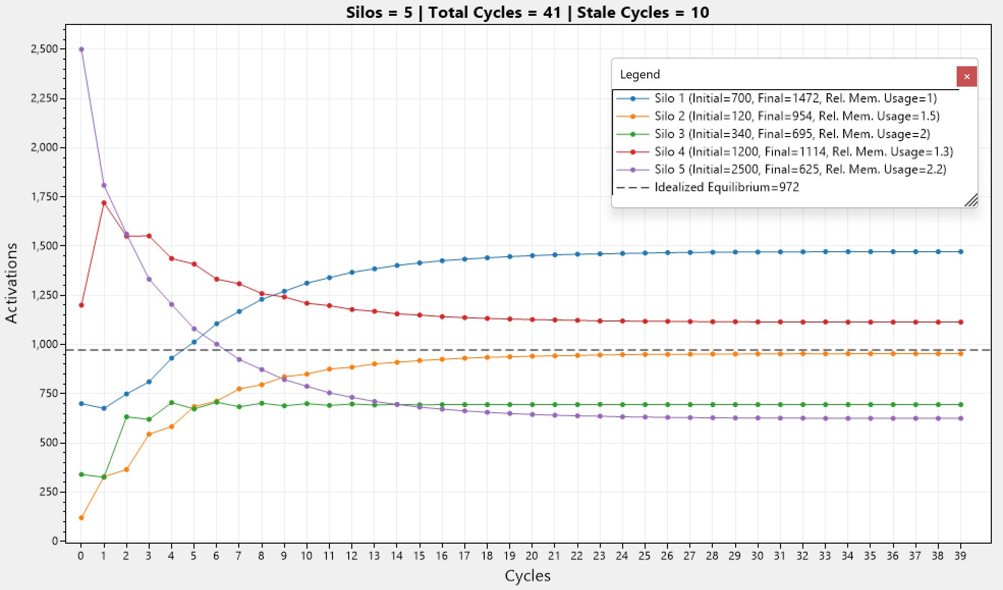
Given the equation for information entropy and our new constraint on the cluster, we can write down the new Lagrangian for our system:
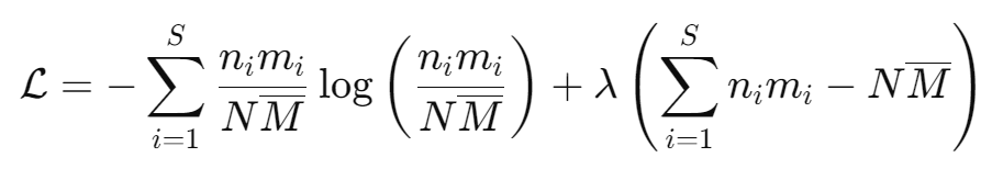
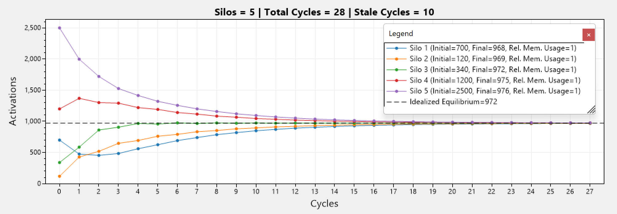
We will not go into a derivation this time as the procedure is similar as the last time, but take it for granted that I did this behind the scenes, and the resulting distribution function becomes:
Each silo gets the average number of activations N/S, scaled down or up depending on how heavy its activations are compared to the cluster’s average. If mi > Mm, silo should hold fewer activations, otherwise it should hold more.
Similarly, the maximum entropy for a perfectly balanced system (where ni mi / N Mm, for all i) is the same as in the unconstrained case:
This is logical as the cluster entropy is independed of any deviation (introduced by different activations and/or memory usages) on the silo level, as we remove the silo boundaries when treating the cluster's entropy.
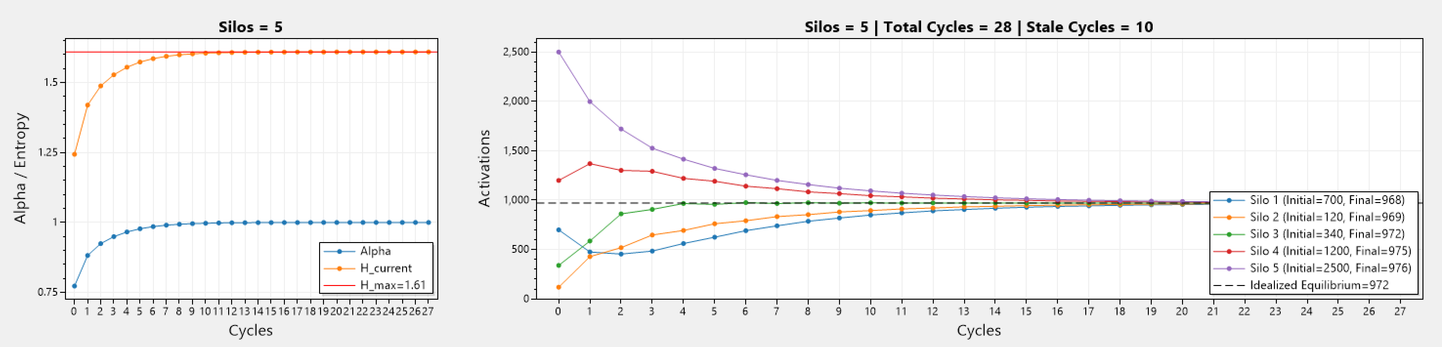
Simulations
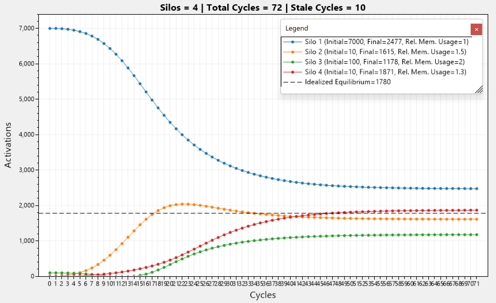
Below we can see a simulation involving 5 silos with different initial number of activations, and different relative memory usages. We can see that constrained equilibrium is reached after 31 cycles and the other 10 are so called "stale" cycles (consecutive cycles yielding no improvement to the current entropy).
Note that the activation count in each silo converges at a different point, away from the idealized equilibrium.
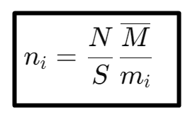
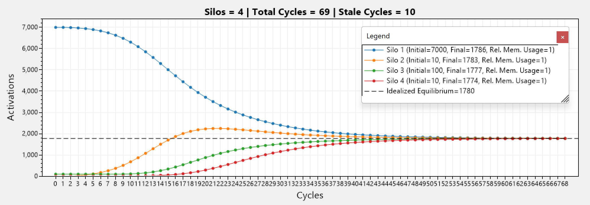
Below we can see that this reduces to the non-constrained version when the memories are all equal. All activation counts converge to the same point, which is the idealized equilibrium.
Adaptive Scaling
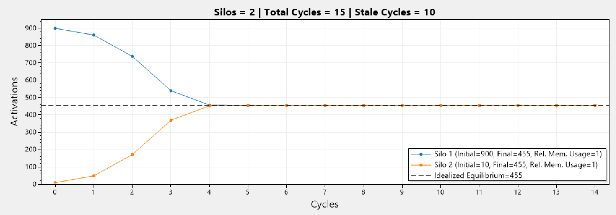
Lets analyze a 2 silo system with different initial activation count for one of the silos. Below we can see a graph that has 900 and 10 activations for silo 1 and 2, respectively. Notice how it took 5 cycles until equilibrium was reached.
Now we have 10x the activation count (from 900, to 9000) for silo 1. Notice how it took 7 cycles until equilibrium was reached. A difference of only 2 cycles for such a major difference in activations.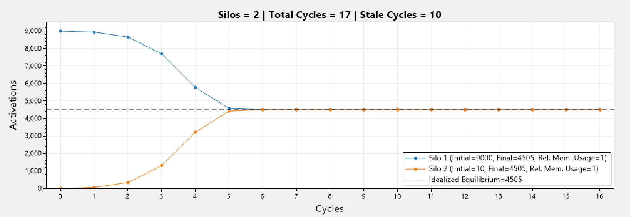
This is due to lack of knowledge on the number of cycles as MAR is working aggressively to reach equilibrium as fast as possible. This behavior is rather unpleasant in real world situations,as it can lead to disruptions in the system when migrating a very large amount of activations at once.
Lets define the growth rate for the cycle component as: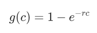
Where c is the current cycle number, and r is some base rate which is user configurable.
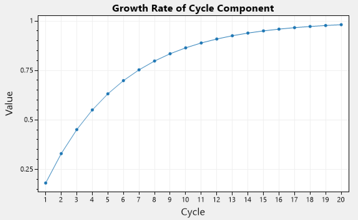
We can see that it increases with each passing cycle. Taking into account that with more cycles passing by, equilibrium is being reached, therefor we can start to increase the migration rate, as by definition there will be fewer overall activations to be migrated.
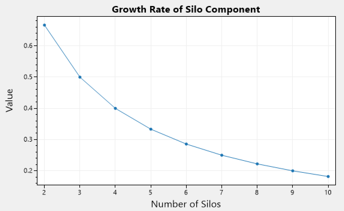
Lets define the growth rate for the silo component as: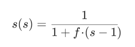
Where s is the silo number, and f is some base rate which is user configurable.
We can see that it decreases with higher number of silos. Taking into account the natural damping that occurs when there are more silos involved as there will be more pairs created to migrate activations between them, therefor we can start to relax the migration rate, as by definition there will be fewer overall activations to be migrated as they are more spread around a higher number of silos.
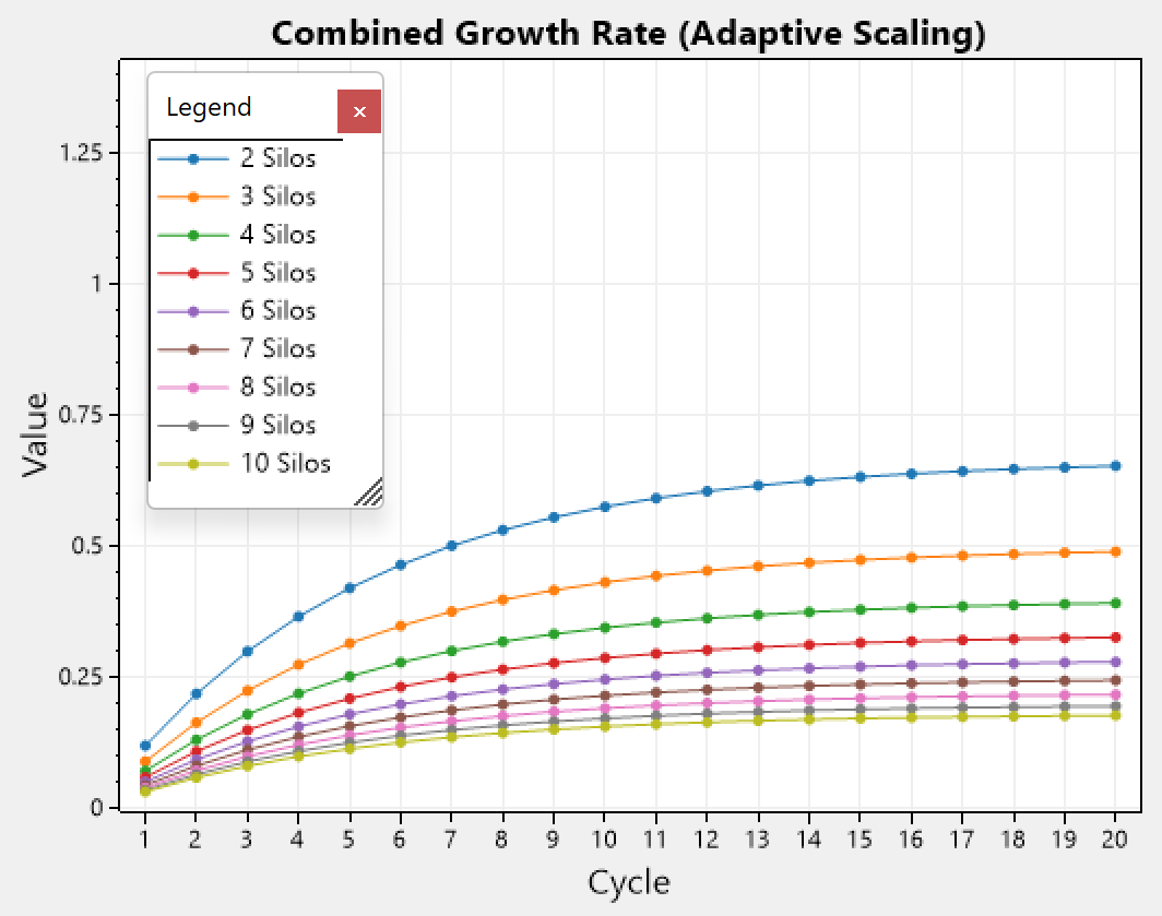
We can create a non-linear combination between the growth rates and define adaptive scaling as:
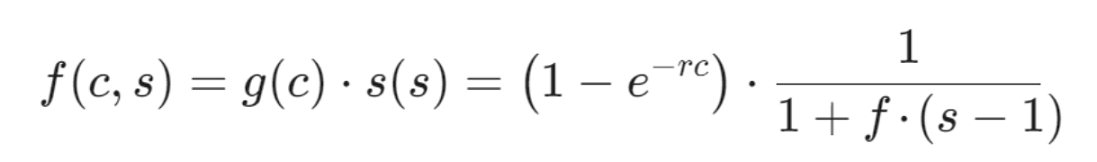
We can see that it initially starts low and gradually increases as more cycles pass by until it stabilizes. In addition, we can see that the overall scaling is lower when the number of silos is higher (different color represent different number of silos). Which is inline with the natural damping of having more silos, and the behavior we generally want to have.
Revisiting our previous simulation, but this time with adaptive scaling incorporated, we can see that the simulation which had [9000, 10] activations now takes 17 cycles to equilibrium, while previously it needed only 7 cycles. This results in a smoother migration rate, and practically reduces the chance of disruptions in the system.
This is even more apparent in a different simulation involving 4 silos:
Just to showcase the same, but this time with varying memory usages.
For reference, here is the corresponding graph that shows how the entropy of the cluster changes as cycles pass by. Although in the above graph we can see tiny fluctuations (in silo 2) the entropy of the system always increases until equilibrium is reached when it hits the maximum entropy possible for the given configuration, and than it stays at that value.
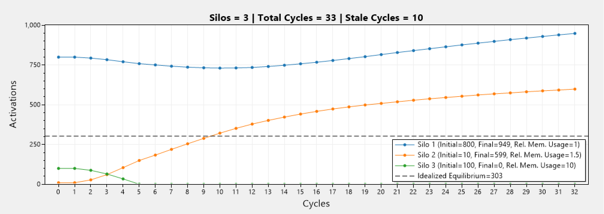
Mean Choice
We have used the harmonic mean because it is particularly effective when we want to understand the "average" in a way that minimizes the influence of large values or outliers.
Lets look at an example where one of the silos has a disproportionately large memory usage (~10x) than the others. Below we can see using the arithmetic mean (commonly know as the "average"). We can see that silo 3 ends up with 0 activations at the end, which in turn ends up diverging the distribution.
This would practically not happen as rebalancing would stop before that, and the .NET Garbage Collector would release the memory, but nonetheless it can be worrisome to know that.
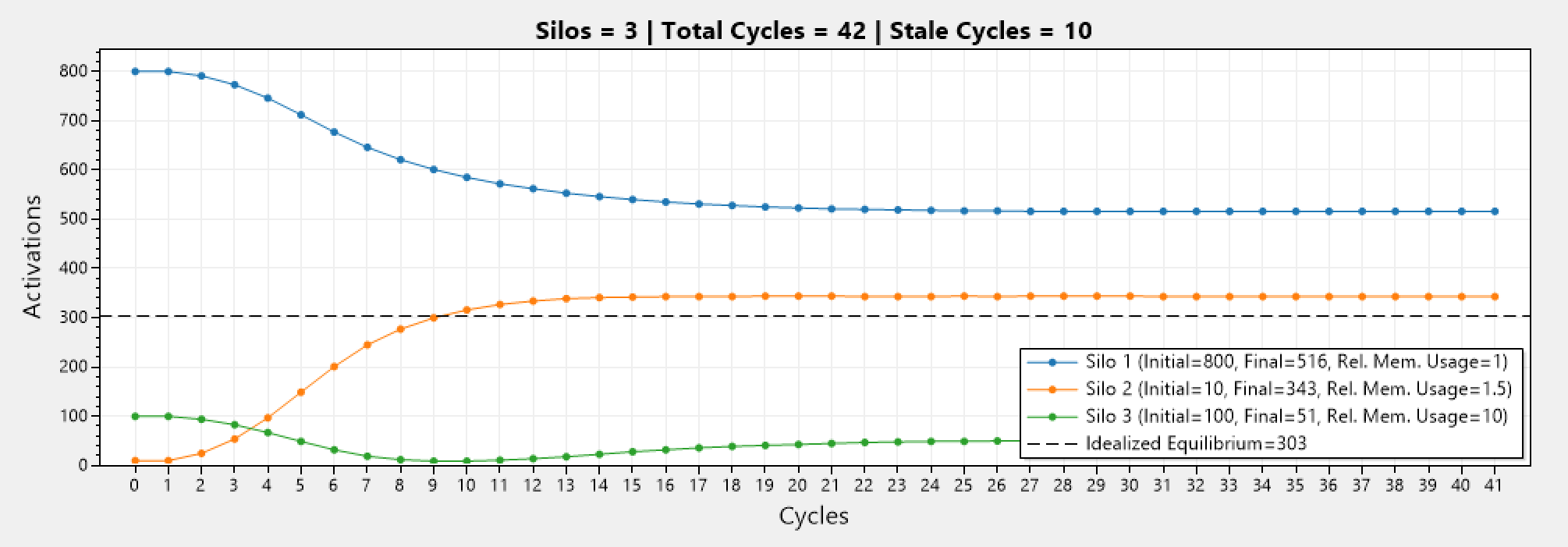
Instead, by using the harmonic mean we can see that silo 3 ends up with 51 activations at the end, and while the number of activations is certainly lower than the other silos (as it should be), nevertheless it is not 0 and the distribution does not diverge.
CPU Constraint
I have chosen not to include a constraint on the CPU usage because unlike ROP, where activations could require placement at a much higher frequency than say MAR's cycle period. In ROP it make sense to use CPU usage as a metric (although it is a filtered version), and even there we are quite pushing it. For MAR the CPU usage would fluctuate too much to be valuable information to incorporate.
Algorithm
Below we have put all we talked about into a pseudo-code that describes the MAR algorithm.
1: while True do
2:     currentEntropy = ComputeCurrentEntropy(cluster)
3:     if currentEntropy < ThresholdEntropy then
4:         equilibriumPoint = ComputeEquilibriumPoint(cluster.activations, cluster.memoryUsages)
5:         pairs = FormSiloPairs(equilibriumPoint)
6:         for cycle = 1 to max_cycle do
7:            if NoReductionInEntropy(x_cycles) then
8:                 break
9:            for each pair in pairs do
10:                optimalActivations = ComputeOptimalActivations(pair)
11:                deviations = ComputeDeviations(pair, optimalActivations)
12:                alpha = ComputeAlpha(deviations)
13:                adaptiveScalingFactor = ComputeAdaptiveScalingFactor(alpha)
14:                avgDeviationDifference = AverageDeviationDifference(pair, deviations)
15:                scaledDeviation = avgDeviationDifference * adaptiveScalingFactor
16:                adjustmentDelta = ComputeAdjustmentDelta(scaledDeviation)
17:                MoveActivationsToLeastLoadedSilo(pair, adjustmentDelta)
18:            end for
19:        end for
20:    end if
21: end while
If you found this article helpful please give it a share in your favorite forums 😉.
The solution project for the simulations is available on GitHub.